
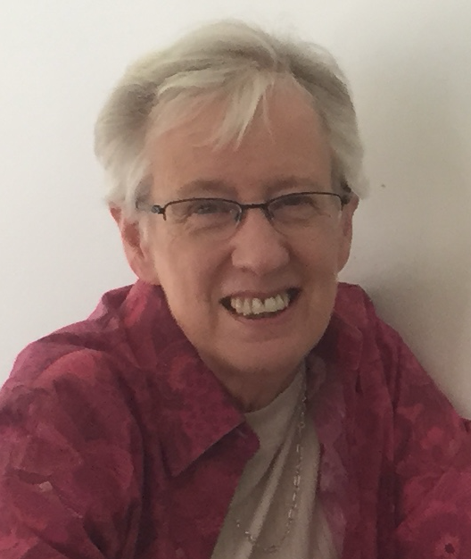
 Jane Watson, University of Tasmania
I am a statistics educator in the Australian state of Tasmania. Recently I collaborated with a Grade 10 math teacher on a unit on statistics and probability to challenge her advanced mathematics class. The students’ backgrounds were traditional and procedural. There were eight extended lessons of 1½ hours using the TinkerPlots software.
[pullquote]…we gave students a variation on the famous Hospital problem: “Ted and Jed are each tossing a fair coin. Ted tosses his 10 times and Jed tosses his 30 times. Which one of them is more likely to get more than 60% heads or do they have the same chance?” Almost unanimously they said, “the same of course.”[/pullquote]
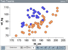
Lesson 1. We introduced students to TinkerPlots in a computer lab working in pairs, starting with the Plot tool. The final challenge we set was to distinguish two of Australia’s “mystery” football codes using height and weight. Figure 1 shows one representation. Students enjoyed the context of the task, with much argument about their favorite code and teams.
Figure 1.
 |
Lesson 2. Then we introduced the Sampler in TinkerPlots for students to experience variation and how long it takes for outcomes of tossing a 6-sided die to even out. They expected to see the frequency distribution of the die even out, but were surprised by how many rolls it took (Figure 2). When we asked what would happen if we tossed two dice and summed them, many expected another “boring” uniform distribution. There was initial surprise, then an “aha” experience.
Figure 2. n = 30, 100, 10000 trials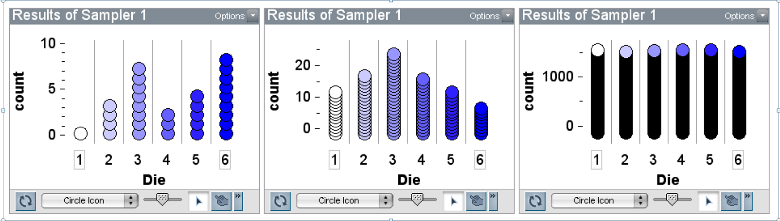 |
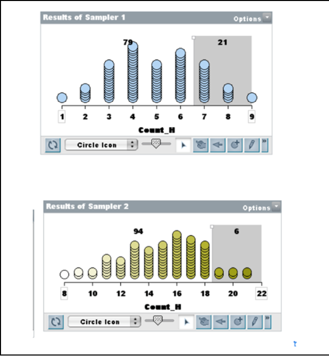
Lesson 3. As the next task using the Sampler, we gave students a variation on the famous Hospital problem: “Ted and Jed are each tossing a fair coin. Ted tosses his 10 times and Jed tosses his 30 times. Which one of them is more likely to get more than 60% heads or do they have the same chance?” Almost unanimously they said, “the same of course.” After creating two Samplers (Figure 3), they accused us of always trying to trick them!
| Figure 3. Tossing 10 or 30 coins, 100 times.
|
Lesson 4. This continued when we asked them what would have happened to China’s population if instead of the historic one-child policy, Konold’s solution of allowing families to have children until the first son was born were implement The main suggestions were: “A population explosion” and “Too many girls.” This problem was again solved with a Sampler in TinkerPlots, using the “repeat until” option and the History tool. Again the result was surprising.
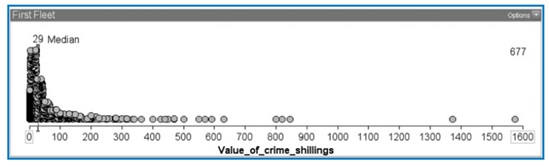
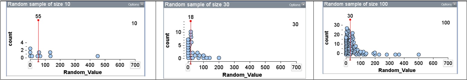
Lesson 5. We then wanted students to experience sampling from a large finite population. We put a population of 677 data points in the Sampler, representing convicts who came to Australia on the First Fleet and the values of the crimes for which they were transported (Figure 4). The students selected samples of size 10, 30, and 100, comparing their variation and medians with the actual population (Figure 5). The students found much variation in the medians of the samples but it decreased markedly as the sample size increased. No controversy here: students were getting the plot!
Figure 4.
 \
\
Figure 5.
Lesson 6. Finally (I hear you say) we moved to resampling as a special case of random sampling where the whole “population” of interest is reallocated randomly to see if an observed difference is unusual or not. The context was an investigation students undertook testing whether it was easier to memorize meaningful or nonsense words (following Shaughnessy’s suggestion). Planning and carrying out the investigation, the students collected the data shown in Figure 6.
Figure 6.
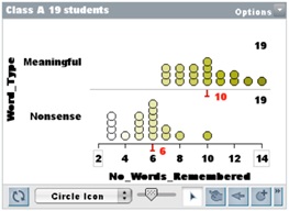
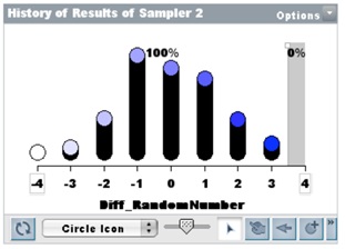
All students basically believed from the start that nonsense words would be more difficult to memorize, hence it was difficult to convince them that this (Figure 6) could be a random outcome if there were no difference in the difficulty of the two conditions. They, however, learned another tool, the Ruler, to measure the difference between the Medians of two sets and apply the History tool to collect the difference in measures for random reallocations of the data. The results for 500 resamples of the data set in Figure 6 are shown in Figure 7, with no results as extreme as theirs in class. Class comment: “We told you so!”
Figure 7.
Lesson 7. The next context considered a very different example, a medical treatment, introduced by Rossman, to add authenticity and use categorical data.
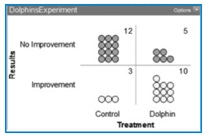
| An experimental treatment for mildly to moderately depressed patients is tested by taking two groups of 15 to the Caribbean. One group swims 4 hours per day for 4 weeks (the control group) and the other group swims for 4 hours per day for 4 weeks with dolphins (the treatment). Ten out of 15 of the dolphin group improve, whereas 3 out of 15 of the swimming only group improve. |
Looking at the 2-way table in Figure 8, it was not as easy for students to claim an obvious “cause-effect” relationship and dismiss the possibility that the result may have happened by chance.
Figure 8.
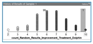
Students put the results (No Improvement, Improvement) into the Sampler and then randomly re-assigned them to the two groups (Dolphin, Control). They saw that when randomly re-assigned, first there might be only 6 people who ‘improve’ by swimming with dolphins, then 4 for the next trial, then 8. When this was done for 100 trials students saw a randomly generated frequency distribution of people who ‘improved’ by swimming with dolphins (e.g., Figure 9). They were much more willing to admit the usefulness of resampling in this case.
Figure 9.
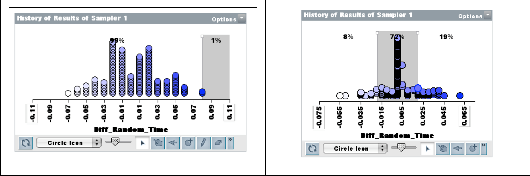
Lesson 8. We felt it was also necessary to give students examples in a context where differences are not always clear-cut. The data were on reaction time of students, comparing two different populations: Boys in Years 5 and 10, and Boys and Girls in Year 10. The data are shown in Figure 10. Collecting 100 random resamples, students could see clearly the difference in the stories told about the medians for the two collections of random samples (Figure 11). They had no evidence for claiming a meaningful difference in Boys and Girls reaction times in Year 10.
Figure 10. Years 5 and 10 (left); Males and Females in Year 10 (right)
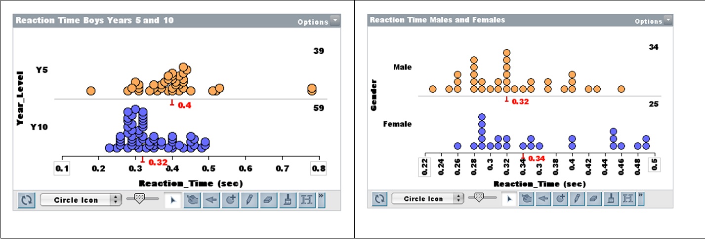
Figure 11. Years 5 and 10 (left); Males and Females in Year 10 (right)
This progression would be helpful to share with high school teachers more broadly, so they can see how simulation can be used over time versus in one stand-alone activity. Simulation is viewed by some as a technology manipultive that you pull out for initial instruction involving conceptual development and then put away so that you can get to the “real content”.
It may be worth pointing out that a pioneer of resampling (well, permutation) inference, E. J. G. Pitman, was also from the University of Tasmania. E. g. https://www.jstor.org/stable/2984124