
 Stephanie Budgett, University of Aukland
At the University of Auckland, our first year statistics course is large. By large we mean about 4500 students per year, with approximately 300 in our summer school semester (lasting 6 weeks, starting early January), 2500 in our first semester (lasting 12 weeks, starting early March) and 1800 in our second semester (starting 12 weeks, starting mid-July). Apart from summer school, we teach in multiple streams with class sizes ranging from 100 students to 400 students per class. Most of our students will not major in statistics and are taking the course because it is a requirement. Over one-half of our students will have taken a statistics course in their last year at school. These students will most likely have taken the Use statistical methods to make a formal inference standard which includes bootstrap confidence intervals. A smaller percentage, say about 20%, may have taken the Conduct an experiment to investigate a situation using experimental design principles standard which includes randomization tests.[pullquote] From a teaching perspective, we believe that the concept of the tail proportion in the randomization test enhances student understanding of p-values.[/pullquote]
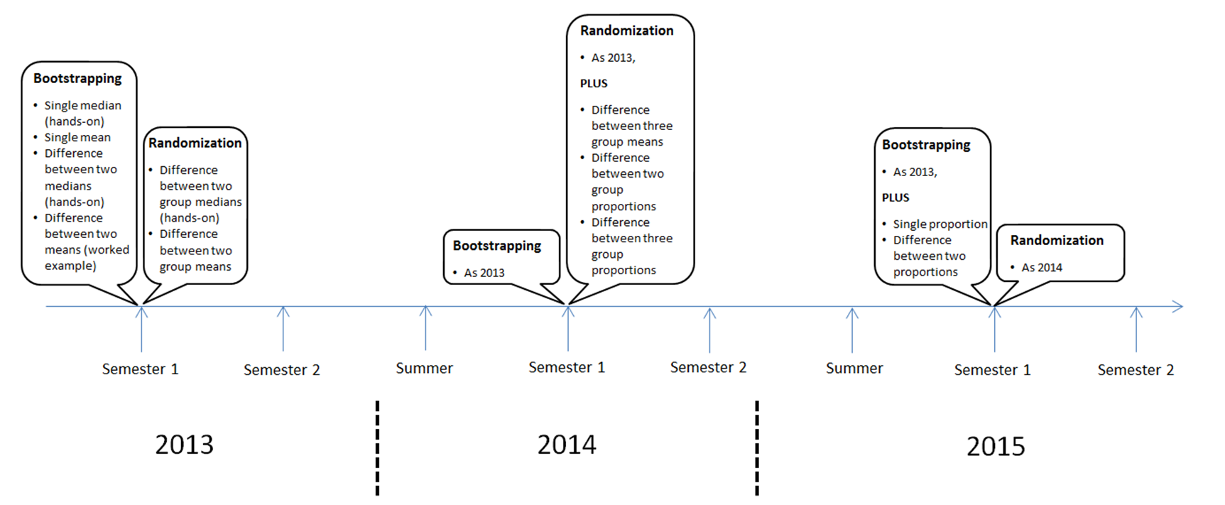
We first introduced our simulation-based curriculum in 2013. Since it was being introduced into schools at the same time, none of our students would have had any prior experience. We hit them with it fast, with two lectures on bootstrapping in the first week and three lectures on randomization tests in the third week. The first bootstrapping lecture involved a hands-on activity for a single median, which motivated the desire to use technology. Using Visual Inference Tools (VIT, see http://www.stat.auckland.ac.nz/~wild/VIT) we then covered bootstrap confidence intervals for a single mean, the difference between two medians, and a worked example illustrating a confidence interval for the difference between two means. A hands-on activity (difference between two group medians) was also used to introduce the randomization test which was then followed an example looking at the difference between two group means using VIT.
In terms of bootstrapping, nothing changed for our second time around in 2014. However, we extended the randomization repertoire to cover the difference between three group means, and also considered differences between two and three group proportions. In 2015 we then extended the bootstrap approach to cover a single proportion and the difference between two proportions.
This timeline illustrates the progression from 2013 through to the end of 2015.
These days we can expect a sizeable proportion of our students to have experienced the bootstrap and/or the randomization test in their final school year. However, it will be completely new to many.
In terms of inferential argumentation, we start by using the randomization test in experimental situations only, with a focus on experiment-to-causation inference. At this stage we take a very informal approach. We do not set up competing hypotheses, and we keep the language simple. In our first use of the randomization test, we compare two group medians and perform a one-tailed test. The resulting tail proportion is small (less than 10%) so we rule out chance acting alone as a plausible explanation for the observed difference and conclude that the treatment administered in the experiment acted alongside chance. We then proceed to comparing two group means, three group means, two group proportions and three group proportions. In all of these experimental situations the tests are one-tailed, and some tail proportions are small (less than 10%) and some are large (greater than 10%).
Given the demands of our client departments, we are unable to remove norm-based inference from our introductory course. When introducing norm-based confidence intervals, we connect the underlying concepts to those of the bootstrap confidence interval. In terms of hypothesis testing, we also link back to the randomization test and build upon these ideas as we introduce more formal terminology. We use the randomization test for a sample-to-population inference situation where the data has arisen from random samples. However, we now take a more formal approach by defining our parameter of interest (difference in means), set up competing null and alternative hypotheses and describe the difference between the two sample means as our test statistic. We then analyze the same sample data using Student’s t-test, making links between our original test statistic and the t-test statistic and between our original tail proportion and the p-value (which are very similar). We then perform further sample-to-population inference t-tests comparing two means and comparing two proportions with an emphasis on the type of conclusion that can be drawn.
Our large introductory course is a popular course which always has excellent course evaluations. Introduction of our simulation-based curriculum does not appear to have changed perception of the course, and the students seem unfazed by the changes. From a teaching perspective, we believe that the concept of the tail proportion in the randomization test enhances student understanding of p-values.