George Cobb, Mount Holyoke College

I’m writing to respond to a pair of questions we often hear from teachers who are considering a simulation-based alternative to the traditional normal-centric course: (1) “If the simulation-based approach is so great, why even bother to teach the normal-based stuff at all?” (2) If I’m going to include the normal-based stuff, do you have any suggestions about how to make the transition? ”[pullquote]The “theory” in what some of us call the “theory-based approach” is the Central Limit Theorem, actually a cluster of theorems about convergence of sampling distributions to normal (Gaussian). [/pullquote]

Why even bother to teach the normal-based stuff at all?

I offer four reasons:

1. Empirical/theoretical: When samples are large enough, many summary statistics have distributions that are roughly normal.
2. Tradition: It’s what almost everybody still does and so you need to know about it.
3. Informal inference: z-scores and +/- SEs are often useful as “quick-and-dirty” approximations.
4. Extensions: Normal based methods generalize easily to comparing several groups at once (ANOVA) and fitting equations to data (regression).

Speaking for myself, depending on the local situation, I’d be inclined to keep these four reasons in mind, and deploy them as seems useful in response to student questions. If you have students who have seen the normal and related inference before, these questions may come up sooner rather than later, and may take the form of “Why bother with all this simulation, when you can just use a formula?” To which I might respond, “Sometimes those formulas can give very wrong answers. We can use the simulation approach to understand when the formula can be trusted.”[pullquote]For Stat 101, the bottom line is that the theorems suggest but do not guarantee that normal-based methods may give good approximations.[/pullquote]

But that’s an aside. I’m trying here to address an opposite point of view: “If simulation is so great …?” I hope (1) – (4) offer a useful approach to answering this question. A related challenge is to help students buy into the transition from simulation to theory-based.

Any thoughts about how to present the transition to theory-based methods?

This is an opportunity (= challenge) for the teacher to help students over a potentially difficult transition. In my experience, such transitions go most smoothly if they are spread out over time and introduced a little at a time. This gradual approach allows students with differing backgrounds and different learning styles enough flexibility to find their own best way. In that spirit, I’ll set out one possible approach, one which I hope you can easily modify to suit your own situation. I’ll start with an overview, then go into more detail.[pullquote]We can use the simulation approach to understand when the formula can be trusted.[/pullquote]

The “theory” in what some of us call the “theory-based approach” is the Central Limit Theorem, actually a cluster of theorems about convergence of sampling distributions to normal (Gaussian). In essence, and informally, these theorems say that when samples are large enough, sampling distributions of some statistics are approximately normal. Note the three weasel-words: large “enough”, “some” statistics, and “approximately” normal. For Stat 101, the bottom line is that the theorems suggest but do not guarantee that normal-based methods may give good approximations. (Making the three weasel-words precise has been a dominant 300-year research theme in probability theory.)

For students in a Stat 101 course, I prefer to stay informal, to emphasize and rely on the three features of a distribution: shape, center, and variability. If the shape of the null distribution is roughly normal, and you know the center and spread, you can use a z-score to estimate a p-value. When it comes to the transition from simulation-based to normal-based, these three features play important albeit different roles.

Shape.

Shape is a qualitative feature, which makes it easier for students to recognize by sight, but harder to quantify. In the spirit of making a gradual transition, you can call attention to the shape of simulated null distributions as soon as they first appear. For example, the null distribution for testing p = ½ will look roughly normal for n as small as 4. Figure 1 shows a simulated distribution with n = 16, p = ½:

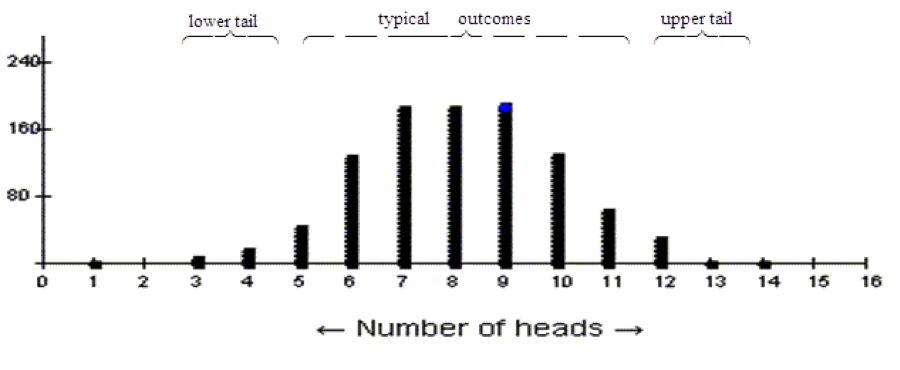 Figure 1: Simulated distribution of the number of heads in 16 tosses of a coin;  n = 16, p = ½

Figure 2 shows another null distribution, this time with p = 1/3 and n = 12:

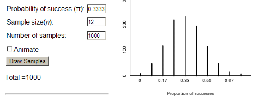
Figure 2: Simulated distribution of the proportion of successes when  n = 12, p = 1/3

After the first few appearances of plots showing roughly normal shape, my inclination is to use shape as a major way to motivate the coming transition: “The same shape seems to be coming up over and over. Can we take advantage of that fact?”

Notes: (a) I’ve used discrete distributions for illustration because many randomization-based expositions start with proportions, and I think it is is a good idea to call attention to the normal shape as soon as it starts to appear. (b) For discrete distributions (i) the smaller the distance between x-values relative to the SD, the more accurate the approximation, and (ii) there is an effective technical adjustment for discrete distributions if higher accuracy is an issue. (c) It’s good to have this knowledge in reserve in case questions come up, but in the spirit of explaining the birds and bees to kids, my inclination is to be open to questions rather than deliver a gratuitous lecture in advance of curiosity.

Center.

For many students it is intuitive that the center of the null distribution of the sample proportion is the null value, so with students willing to speak up about their conjectures, all you need to do is to confirm that they have articulated a provable fact.

Variability.

Assume a normal shape for the null distribution of the sample proportion, with mean at the null value. All you need for a z-score and approximate p-value is the SD. Unfortunately, the formula for the SD of the sample proportion is almost impossible to make simple and intuitive for students at this level. (It can be done, slowly and empirically, but it takes about a week of simulation activities and discussion. Not a good use of time.) So the formula for the SD must be something of a deus ex machina. (Don’t apologize: exploit the opportunity to evangelize for taking a more advanced course.)

Once students have shape, center, and SD, then z-scores and the standard normal are just a step away.

Final thoughts about the transition.

My own inclination is to lean heavily on shape, center, and SD, and on the resulting z-scores and p-values, as above. The fact that the results are at best only approximate is critical, but the specific validity conditions are also at best only approximate, and their specificity can be a trap for students who want rules to memorize. What matters much more is the general principal that you can use simulation as a check on the normal approximation.